Saw #11: Building a Tiny Mixture of Experts Microscope

The mixture-of-experts models worth reading about have hundreds of billions of parameters, and the ideas inside them are hard to see at that size. A router chooses six experts out of 256, forty-three times per token, and what you can observe from outside is a throughput number. I wanted to watch the mechanism, not the number. So I built one with 7,096 parameters.

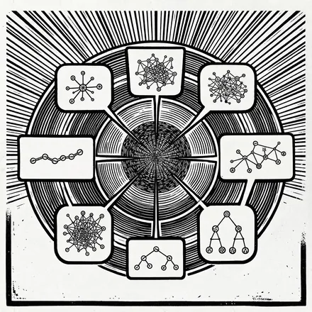
moe-microscope is an sw-MLPL project that builds a tiny mixture-of-experts language model, MicroMoE, from scratch, and lets you look inside every part of it. Each mechanism is a separate, executable lesson that records its own intermediate values, draws them, and measures memory, speed, and quality against a dense baseline. You read the MLPL, change it, rerun it, and watch the numbers and pictures change.

Resource	Link
Live demo	sw-ml-study.github.io/moe-microscope — the lessons, frame by frame
moe-microscope	sw-ml-study/moe-microscope · wiki · results
Campus	Software Wrighter Research Campus — the docent is here
sw-MLPL	sw-ml-study/sw-mlpl · playground
FreeToken	FlashML-org/FreeToken — the inspiration
Prior posts	TRM · HRM · Engram · Engram revisited
“Sharpen the Saw”	The 7 Habits of Highly Effective People (Stephen Covey)
Comments	Discord

Why “Saw”? The name is Habit 7 from Stephen Covey’s The 7 Habits of Highly Effective People: stop cutting long enough to sharpen the blade. This series is where I routinely add tools and improve the ones I have, on the principle that time spent on the tools comes back many times over in everything built with them. This week two blades are on the stone at once: the microscope is a new tool for examining mixture-of-experts implementations side by side, and building it is how sw-MLPL, the language underneath, gets its next set of fixes and features.

Why build it

Two reasons, and the repository exists for both equally.

A workbench for tiny models that are going to leave the laptop. The first stop is the browser, where the lessons already play back frame by frame, and where a model of a few thousand parameters is small enough to run — and eventually train — in front of you. The end of the road is a microprocessor with something like 256 MB of RAM and half a TOPS of neural accelerator — a LicheeRV or SG2002-class board, not a GPU. A model that fits there is not a shrunk-down copy of a big one; it is a different set of trade-offs, where memory bandwidth and the cost of launching an expert matter more than arithmetic throughput. I want a place where those trade-offs can be tried at a scale that runs in seconds on a CPU, measured honestly, and then carried down. The same source runs at microscope scale (CPU, seconds, thousands of parameters) and, under device("mlx") { }, at lab scale. The embedded board is an inference target for the packed model file, reached by a later runtime, and every design decision here is made with it in view.

Dogfooding sw-MLPL. A language for machine learning is only proven by writing machine learning in it, and a mixture of experts is a demanding program: a router trained through a gate, a list of models updated by one optimizer, weight sharing across recurrences, gather and scatter on the autograd tape, distillation losses, packed byte I/O. Every place where the language got in the way has become a minimal reproducer, a pinned probe that fails loudly when the upstream fix lands, and a work order for sw-mlpl. Sixteen of those have been fixed upstream so far — softmax arity on the tape, user functions inside grad, differentiable gather_rows, repeat inside a traced function, one_hot and argmax as stop-gradient constants, a loud error instead of a silent zero gradient, index arithmetic inside a traced scope — and the first four were fixed the day they were filed. Seven are open, including two the docent work turned up this week. The model got better and so did the language, which is the point of dogfooding.

The four ideas, at one tiny scale

MicroMoE combines four ideas that normally live at very different scales:

• Sparse routing over a bank of small experts: only the top-1 or top-2 experts run for each token, so total parameters and active parameters come apart.
• Recursion, from HRM and TRM: one shared block applied several times, so reasoning depth is bought with repeated compute instead of unique layers.
• Conditional memory, from DeepSeek’s Engram: the last two or three tokens are hashed to a slot in a table and the stored vector is added through a learned gate, so plain memorization leaves the neural network.
• Residency, from FreeToken: a mixture of experts solves the compute problem but not the storage problem, so treat memory as a hierarchy and keep an expert cache that follows the router’s actual choices.

Those are four independent kinds of sparsity — parameter sharing, conditional compute, conditional memory, residency — and each is a separate switch with its own lesson that turns it on alone against the dense baseline. That is the design decision that makes the project a microscope rather than a demo: you can ask what recursion buys without also changing the experts, or what an expert cache costs without also changing the model.

                   token ids
                       |
             +---------v---------+
             | token embedding   |
             +---------+---------+
                       |
      recent ids ------+------------------+
                       |          +-------v-------+
                       |          |    Engram     |  hashed 2/3-gram rows,
                       |          |  lookup+gate  |  projection, learned gate
                       |          +-------+-------+
                +------v------------------v------+
                | shared recurrent block         |<----------+
                | rms_norm -> causal attention   |           |
                +---------------+----------------+           |
                         +------v------+                     |
                         |   router    |  logits [T, E]      |
                         +------+------+                     |
                                | top-k mask, gate           |
                         +------v------+                     |
               RAM/file--|expert cache |  LRU over (block,   |
                         +------+------+  expert), bytes     |
                 +--------------+--------------+             |
              expert         expert         expert          |
                 +--------------+--------------+             |
                            combine                          |
                          state update ----------------------+  R times
                                |
                             LM head

What you can watch

The live demo: each lesson's recorded frames, stepped in the browser.

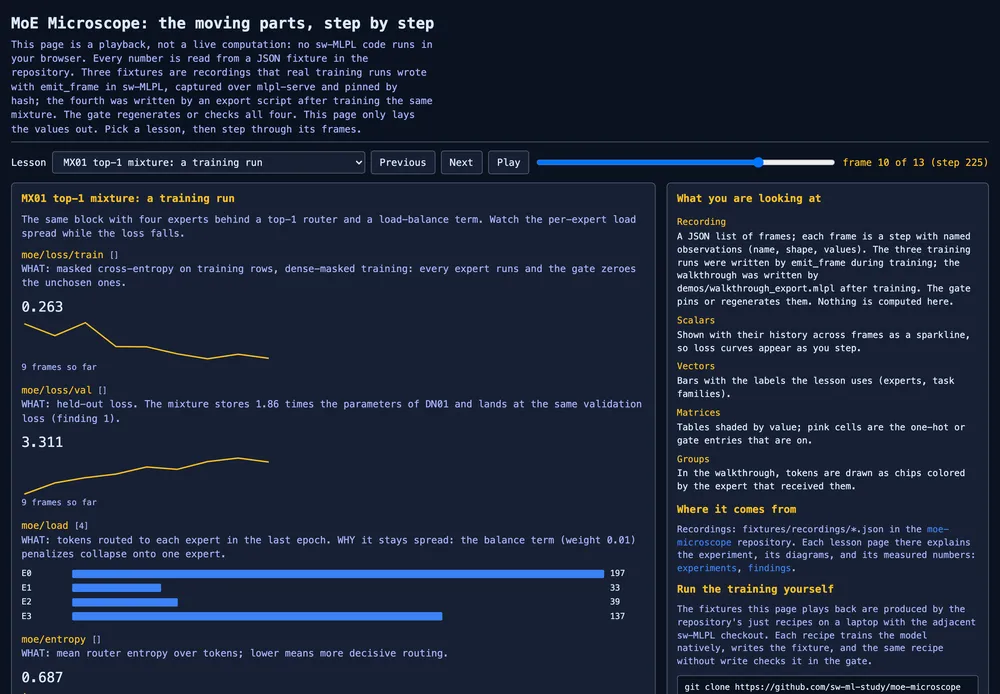
Every lesson records its intermediate values as named frames while it trains, and the live demo plays those recordings back in the browser: pick the dense baseline, the top-1 or top-2 mixture, or one window through routing and dispatch, and step through the frames — the loss as a sparkline, per-expert loads as bars, routing matrices shaded by value, tokens as chips colored by the expert that received them. It is a playback, not a live computation: no sw-MLPL runs in the page, and every number it draws was written by a real training run and pinned by hash in the repository. The same recordings are what the generic Rust/Yew/WASM host renders.

The domain is deliberately small: small-integer arithmetic, rev/sort sequence transformations, tiny MLPL expressions checked against the interpreter itself, and short templated prose. Fifty-two symbols, windows of twenty-eight tokens. Each example carries a task tag the model never sees, which is what makes the interesting question measurable: do the experts specialize, and along what lines?

The router, before training: logits, probabilities, the one-hot choice, and the gate that keeps the chosen expert's probability so the router still gets a gradient.

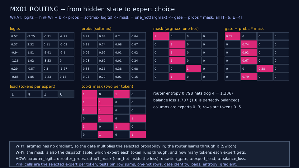
The router is one small linear layer. A token’s hidden state goes in, one score per expert comes out, the top-k win. The choice itself is an argmax with no gradient, so the gate multiplies the chosen expert’s probability into the output — if raising that probability would have lowered the loss, the router raises it. A load-balance term keeps the first expert that gets slightly better from taking every token, which is otherwise exactly what happens.

The specialization map. For each task family, the share of its tokens each expert received. The router never saw a family tag; any structure here is emergent.

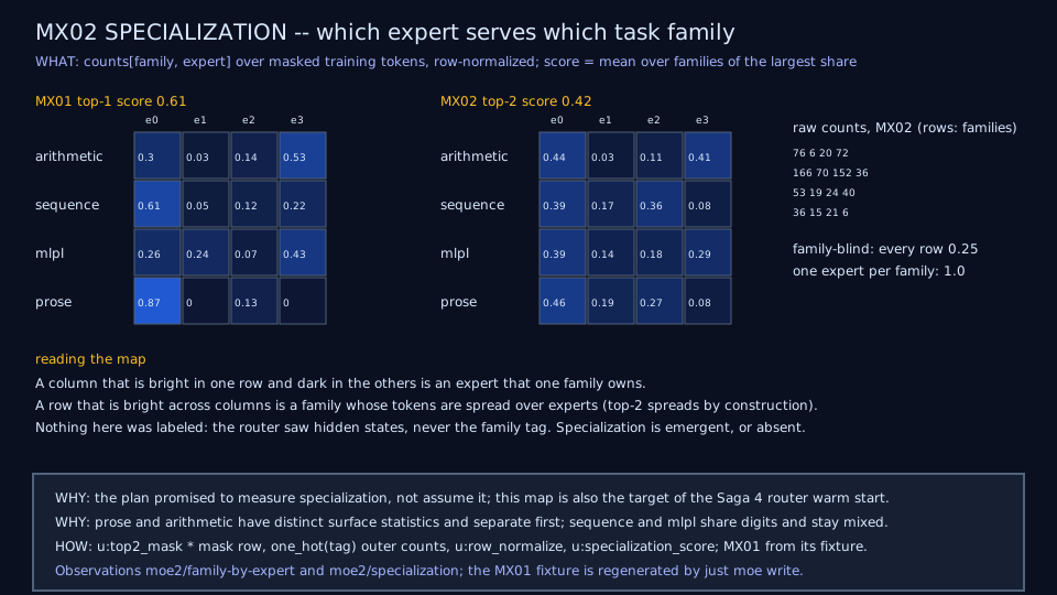
Nobody labels an expert “the arithmetic expert.” Specialization is an emergent property of routing plus gradient, and it is not guaranteed — experts can just as easily split tokens by position or frequency. So the project measures it instead of assuming it. The specialization score is the mean, over families, of the largest share any one expert takes; 0.25 would mean routing ignores the family entirely. Under top-1 it is 0.61: prose and arithmetic each lean on one expert. Under top-2 it is 0.42, because spreading each token across two experts spreads the map by construction.

The numbers, honestly

The dense baseline is one transformer block, 3,812 parameters, trained in sixteen seconds. Replacing its feed-forward layer with four experts and a router gives 7,096 parameters stored — 1.86 times as many — while a token touches 3,064, or 1.02 times as many, at the same validation loss. That is the entire promise of a mixture of experts in one row of a table: capacity grows, and the cost per token does not.

Three more results are the kind you only get by being able to see everything:

Sparse dispatch is exactly the dense model. Training runs every expert and lets the gate zero the unchosen ones, which keeps autograd simple. Inference gathers each expert’s routed rows, runs the expert once on that sub-batch, and scatters the results back. Over 120 windows the two outputs agree to the last bit, while expert row evaluations fall from 13,440 to 3,360. And one honest number alongside: in this interpreter the sparse path is slower per window, 0.74 ms against 0.42, because gather, scatter, and loop overhead cost more than the three tiny matmuls they skip. The saving is real in the counts and becomes wall-clock time only with larger experts or a compiled runtime, which is why the results table records counts first. The generation benchmark says the same thing from the other side: roughly 6,000 tokens per second dense, 3,200 top-1, 2,000 top-2, and 3,100 for packed delta experts, all with p95 token latency under 0.6 ms on one laptop.

Experts can be much cheaper than you think. Instead of four full experts at 1,072 parameters each, sixteen experts as rank-4 deltas over a shared feed-forward layer — 128 parameters apiece, all sixteen packed into two matrices so the routed sum is two matmuls. That configuration has the best validation loss in the table, with 2,048 expert parameters against 4,288. Hundreds of experts become affordable, and the big shared matrix stays static, which is exactly the shape a small accelerator likes.

Data is the lever. Epochs are not. At 120 training examples, doubling the epochs makes validation loss worse for both models, while eight times the data cuts it by two thirds and turns prose into a solved family. The mixture beats the dense model at 480 examples and loses at 960 at twice the training cost, which is the honest state of a four-expert model on this domain.

Every one of those numbers is labeled measured, derived, or estimated in a resource budget whose calculator is pinned to the lessons’ own parameter counts. One full expert is 8,576 bytes at f64 and 536 bytes of INT4 payload. The whole four-expert model is 55 KiB.

A docent for the campus

The campus with the docent open. Try it.

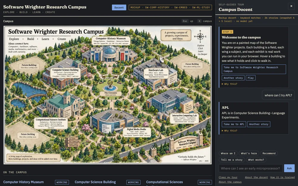
A synthetic domain is the right place to learn the mechanism, and the microscope’s first real domain came from the Software Wrighter Research Campus — the isometric map of the public work from last week’s post. Every lobby has an easel, and underneath the featured exhibit you can ask a docent where something is: “where can I try APL?”, “show me an early microprocessor.” The docent on the campus today is deterministic — an alias-and-concept matcher over the catalog with keyword rules for intent — and the question the microscope was asked is whether a trained model would do better.

The setup is the honest part. The catalog is the corpus: every place carries a reviewable docent block — aliases, concepts, authored questions, a few canned stories, and a one-line status with a maturity level — and a deterministic generator turns it into 965 labeled rows across six intents (navigate, explain, recommend, story, status, unsupported) and twelve destinations. Nothing about the campus lives in weights; a model only has to say what the visitor wants and where to send them, and the catalog supplies the title, breadcrumb, and URL. A separate set of 54 paraphrases — phrasings that contain no alias verbatim, plus off-topic questions — is never trained on. That set is where a model has to prove it is worth shipping, against a bar written down in advance: twenty points better than the matcher on paraphrases, for both destination and intent.

The first trained docent is a flat dense classifier, 26,003 parameters over hashed word and bigram features: 0.925 destination accuracy and 0.938 intent accuracy on held-out rows that share the training templates. On the paraphrases it scores 0.296. The matcher, with zero parameters, scores 0.685 on the same paraphrases, rejects every off-topic question where the model rejects three in ten, and wins on destinations outright. The docent beats it only on intent, where keyword rules are crude. The bar was not met, by thirty-nine points in the wrong direction, so the campus keeps its deterministic docent, exactly as the plan said it would if the margin fell short.

That is a decision about the campus, not about the microscope — the tool exists to learn and build MoE models whether or not the campus ever needs one — but it is a good week’s result for a tool whose job is to measure rather than assume. It also says precisely where a model would earn its place: the matcher’s paraphrase score comes from words the catalog already holds, and hashed features cannot generalize from them. The next two experiments attack exactly that, and both are ongoing research rather than shipped: word vectors from the campus’s own text held in an Engram-style table, so aliases and near-terms live in cheap deterministic memory, and then routed experts over the same features. Each is measured against the matcher’s column; if the margin is still not met, the matcher stays.

The campus also holds the microscope’s best future experiment in reserve. The IBM 1442 card reader and its radio demonstration are deliberately left out of the catalog snapshot the docent was trained on. When they arrive, the catalog will know at once and a trained model will not — the world changed, the application’s data knows it, the model doesn’t — and the retraining, and whether it costs the model anything it already knew, becomes a measurement rather than a story.

What is still to come

The lessons that exist today are the dense baseline, routing, top-1 and top-2 mixtures, sparse dispatch, low-rank delta experts, the data-scale sweep, an in-repo teacher for distillation, the resource budget, the generation benchmark, and the campus docent’s corpus, first classifier, and matcher baseline. Ahead are the parts that connect most directly to the embedded target: recurrence, the from-scratch Engram with a table-size sweep, distillation at four levels, INT8 and INT4 experts, the capacity-limited expert cache with its hit-rate curve, the CPU/NPU hybrid split, and the packed model file that has to fit in 256 MB — and, on the docent side, the word-vector and routed-expert models that have to beat the matcher before anything changes on the campus.

Every one of those is a question with a measurement attached, and every measurement lands in the same table as the ones above. The documentation is organized around that table as three reader journeys — I want to understand the idea, I want to know whether it works, I want to modify or reproduce it — with one concept page per mechanism, one laboratory report per experiment, and a results dashboard that states each finding as evidence, interpretation, and limitation. The wiki mirrors the same hierarchy.

Building the smallest useful mixture of experts was never the goal. The goal is to be able to look inside one — and to have somewhere to stand when the next tiny model needs to run on something small.