Made Visible #4: Rosetta M, a Stone with Four Faces

Part 1 drew a microkernel’s flash. Part 2 drew a conventional kernel’s frames and mappings. Part 3 drew resident model state. This one draws no system at all — it draws a notation that does not exist yet.

Rosetta M is a mock-up of a proposed array language for machine learning, shown the way the Rosetta Stone shows a decree: the same thing in more than one script. Here the scripts are the mathematics as a paper writes it, one line of proposed notation, a live dataflow, and, when the computation trains, its loss trace — four faces of one stone, with training time as the axis they share. There are ten stones, one per small computation. The convolution from Machine Learning #9 is the one this post turns first, because that post ended by asking what the notation would have to look like.

Resource	Link
The mock-up, live	sw-ml-study.github.io/m-poc — already training when it loads; drag the stone to turn it, pick a stone from the drop-down
The source	sw-ml-study/m-poc — the records, the renderer, the capture scripts
The engine	sw-ml-study/sw-mlpl — every number on the page came out of it
The worked example	ML #9: Teaching an Array Language to Say CNN and Zhao, Wang, Wang & Liu, Algorithms 11(10):159, 2018
Comments	Discord

One stone, turning: math, notation, dataflow, trace --- four faces of one computation. This is the CNN stone; the other nine turn the same way.

On the live page: the drop-down picks a stone; 0 resets the view and sets it rotating; 1–4 turn one face to you — math, notation, visualization, trace; a toggles auto-rotate; w lays every face side by side; hover any symbol and its callout appears.

Turn a stone slowly and the faces come round as math, notation, visualization, trace, math again — the way you’d read a paper, write an implementation, watch it train, then check the loss. The mock-up’s wager is that those are not four activities. They are four faces.

One record, four faces

The Rosetta Stone carries one decree in three scripts, and the script people could already read unlocked the two they could not. Rosetta M borrows the arrangement. The script everyone can read is the mathematics, written the way the literature writes it. The script being proposed is M: one line of array notation in the APL2 tradition, extended with the glyphs machine learning keeps needing — sliding windows, named-axis reductions, gradients. The third and fourth faces are the check that the two scripts say the same thing: the computation drawn as dataflow with live numbers moving through it, and, for the stones that train, the loss they report as they go.

Every stone is one equation record — a list of symbols, each with a role, a name and a one-sentence doc, and per face an ordered list of tokens that render it. = on the math face and ← on the M face are the same symbol; so are ² and *2. Click a symbol on any face and its callout appears, the same callout whichever face you clicked it on, because there is only one symbol. The M face is proposed, not run: there is no parser and no evaluator, and the glyphs are placeholders. Everything that executes is sw-MLPL, which renders the faces from the record, trains the stone with its autograd, and emits the trace and geometry the page replays.

The four faces below belong to the CNN stone, because that is where ML #9 left off. Each of the other nine has the same faces and the same callouts.

Face 1: the math, with every symbol willing to explain itself

Face 1, Math: the triple sum, walking its symbol callouts.

This is Zhao et al.’s definition of one output cell, unchanged — and the capture beside it walks the callouts: r selects the output filter, ∑ binds the summation, q runs over input channels up to Q, u and v step across the kernel window, W is the kernel, X the input, and x, y fix where the window’s top-left corner sits in the input. On the live page these callouts are not a video — you click any symbol and it explains itself; the capture just walks the clicks for you.

               Q      M_w    N_w
  y[r,x,y]  =  ∑      ∑      ∑     W[r,q,u,v] · X[q, x+u, y+v]
              q=1    u=1    v=1

Face 2: the same thing, one line of M

Y ← +/[channel,kernel-y,kernel-x] W × ⧉[Mw,Nw] X

Face 2, M: the same convolution as one line of proposed notation, walking its callouts.

Read right to left, as array-language tradition demands. ⧉[Mw,Nw] X gathers every sliding kernel-window of the input at once — the window rearrangement from ML #9. W × multiplies each window by the kernel, the kernel broadcasting against the stack of windows. +/[channel,kernel-y,kernel-x] sums the three named axes away in a single pass — one reduction, three axes, no loop nesting. Y receives the whole output map at once; there is no [r,x,y] subscript because there is no cell, just the map.

The glyphs are placeholders, the notation is proposed, and nothing here runs — the mock-up renders the faces from one equation record and sw-MLPL does all the actual arithmetic. The three nested Σ’s of face 1 have become one / with three names after it. That collapse — the paper’s whole loop nest into one reduction — is the entire argument for an array notation in one line.

Face 3: what it does, while it trains

Face 3, Visual: the dataflow, animating through training.

The third face is the computation itself: input, windows, kernel, multiply, reduce, output, loss — drawn as dataflow and animating through sixteen epochs of gradient descent, the numbers coming from sw-MLPL’s autograd as it trains the kernel. Scrub the epochs on the live page and the data moves while the equation and the notation sit still: the two things face 1 and face 2 are saying are exactly the thing face 3 is doing.

Face 4: how it went

Face 4, Trace: the loss, drawing itself down as the epochs pass.

The fourth face is the one that is about how it went rather than what it is: the loss, drawn over the epochs, falling as the kernel learns. The other three faces show the computation from the outside — its mathematics, its notation, its dataflow. The trace face is the computation’s own report: here is what training felt like from inside, one number per epoch, going down and to the right.

Five of the ten stones carry this face. A memory map never needed one; a training loop does.

The drop-down: ten stones, one argument

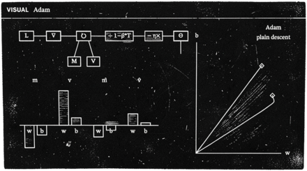
The CNN stone is the one this post turned first, but it is one of ten in the drop-down, and the ten are ordered the way they are for a reason. The block print at the top of this post, for instance, is the Adam stone’s thumbnail — it comes last on purpose.

The drop-down, in tour order. Reading left to right, top to bottom: one neuron, feature normalization, dot product, matmul, softmax, image normalization, the CNN, the sigmoid neuron, attention, Adam.

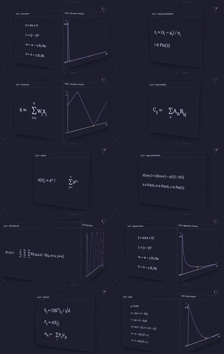
First the headline stone, then a notation ladder that climbs from pointwise arithmetic to three nested sums, then the variants — a squashing function, an attention composed from stones you have already met, an optimizer with a memory:

Stone	Says	Why it is in the drop-down
One neuron	Ŷ ← B + W×X	The headline: a linear fit trained by gradient descent, the whole story in miniature — equation, notation, dataflow and its fourth face, Trace, the training loss over time.
Feature normalization	Z ← (X − Μ) ÷ Σ	The bottom rung of the ladder: the simplest rule on the page, each feature centred and scaled, every position on its own — no windows, no reductions yet.
Dot product	S ← +/ W×X	The atom: one multiply per pair, one running sum. Every reduction after it is this stone in a costume.
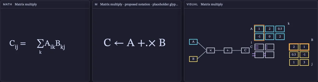
Matrix multiply	C ← A +.× B	The workhorse: every cell of C is the dot product of a row and a column. The whole ladder rung exists to make attention legible later.
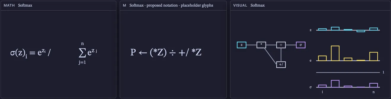
Softmax	P ← (*Z) ÷ +/ *Z	Scores into probabilities: exponentiate, divide by the sum. Pointwise arithmetic wrapped around one shared reduction.
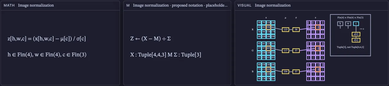
Image normalization	Z ← (X − Μ) ÷ Σ over a 4×4×3 image	The lift: the feature stone’s rule applied to a whole image, the per-channel means and spreads broadcast by an index projection, never copied. This is the rung between pointwise and windows.
CNN triple sum	Y ← +/[...] W × ⧉[Mw,Nw] X	The top of the ladder, this post’s stone: three nested sums become one named reduction over a window gather.
Sigmoid neuron	Ŷ ← σ B + W×X	The first variant: the headline neuron with a squashing function between fit and loss — the training loop has to differentiate through σ.
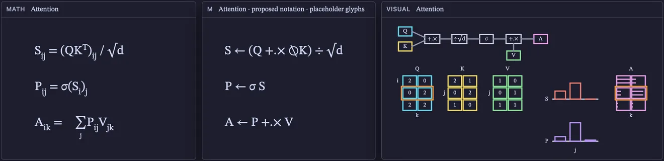
Attention	S ← (Q +.× ⍉K) ÷ √d, P ← σ S, A ← P +.× V	The composition: two matmuls and a softmax — nothing new, only stones you have already seen, assembled into the transformer’s core.
Adam	Θ ← Θ − η×M̂ ÷ √V̂ + ε	The optimizer with a memory: a running mean of the gradient and of its square, so every step is about the same size whatever the gradient’s scale — gradient descent that carries its own context.

Five of the ten — one neuron, dot product, CNN, sigmoid, Adam — carry the fourth face: Trace, the training loss drawn over time, the only face that is about how it went rather than what it is. The other five are about the computation itself, and the drop-down is shaped like the argument: from one rule you can see whole, to one reduction that took the array-language world thirty years of vocabulary to say in a line.

What this is, and is not

This is a mock-up — ten stones whose faces are the math, the notation, the live structure, and the training trace of one small computation each, with time as the axis they all share. It points at a language we have not built and are not naming yet beyond the placeholder: a visual programming language in the APL2 tradition, extended with the glyphs machine learning actually needs — windows, named-axis reductions, gradients — where the program, the mathematics it encodes, the data flowing through it, and the story of its training are four views of one object rather than four artifacts kept in sync by discipline.

The series’ three-layer split holds here too: the renderer knows nothing about machine learning, the equation knows nothing about rendering, and an array language sits in the middle turning one into the other. There is no parser, no evaluator, no repository, and no name. There is a page, and every symbol on it has a callout.

---

The ten stones, side by side

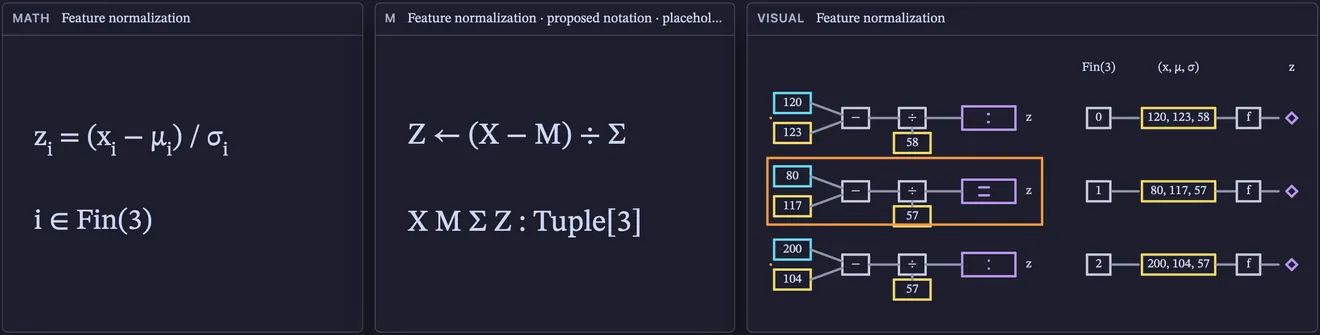
The live page has one more view: its View row (key w) lays every face of a stone flat in a row, all of them live — the Rosetta Stone as a strip rather than a block. Here is that row for each of the ten stones, in tour order — click any one to open it at full size, every face playing through its time axis at once; click the background, press Escape, or hit the × to come back.

1One neuron 2Feature normalization 3Dot product 4Matrix multiply 5Softmax 6Image normalization 7CNN triple sum 8Sigmoid neuron 9Attention 10Adam

×

×

×

×

×

×

×

×

×

×