Array Languages #11: Math Equations as X_eTaL Macros

ML #9 ended with a CNN’s triple sum and a question: what notation could say it in one line? Post #5 said experiments were under way with macros for ML equations. This post is what they produced: a library, Equations. Its purpose is to let one equation be seen three ways and to move freely between them: as the math a paper prints, as an X_eTaL macro call that reads almost the same, and as the ordinary X_eTaL the macro expands to and runs. Because the typeset math and the running code come from the same call, they cannot drift apart.

Resource	Link
The design	docs/spatial.md — the call, the lowering, the errors, the expected outputs
The library	Equations in X_eTaL-libraries · its reference
Try it	the live demo: pick Equations, run the CNN demo, see the math drawn
Why this call	docs/eq-rationale.md — seven ways to write it, compared
The thread	ML #9 · Array Languages #5: X_eTaL-ML
Comments	Discord

One equation, three views

One equation, three views: the math, the macro call, and the X_eTaL it expands to. Click to enlarge.

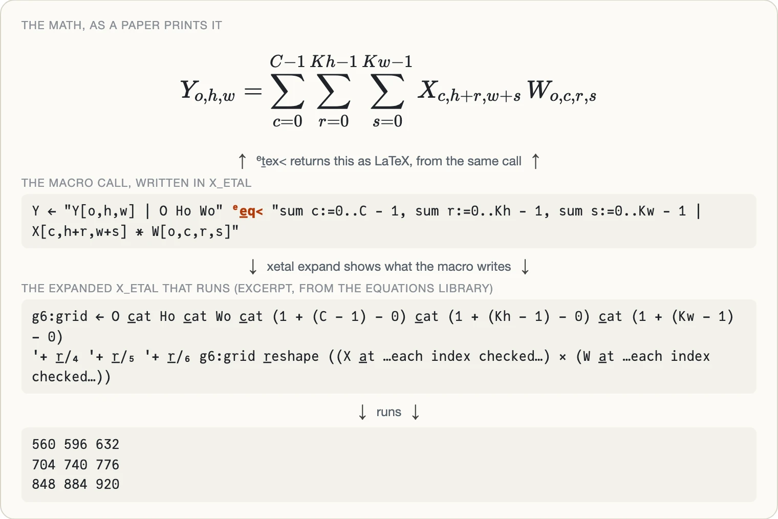
Machine-learning papers are written in math, and programs are not. Translating one into the other by hand is where mistakes hide: an index off by one, a sum over the wrong axis, a bound that is right in the paper and wrong in the code. The equation macros keep the two together. The figure shows the three views of one equation, the convolution a CNN computes:

• The math, at the top, typeset as a paper would print it. It is not drawn by hand: the macro returns it as LaTeX, from the same call that computes the value.
• The macro call, in the middle, which is what a programmer writes. It reads almost like the math: the same indices, the same bounds, the same summand.
• The expanded X_eTaL, below it, which is what actually runs, plain array operations that xetal expand will show to anyone who wants to check the macro’s work.

Read up, and the code can be checked against the paper. Read down, and the paper becomes a program, with its answer at the bottom. All three come from the Equations library: the math is the LaTeX it returns, the expansion is what xetal expand prints, and the answer is what the expansion computes.

Macros first, syntax only when justified

An ML-focused language could add notation for sums to its grammar. The approach here is the opposite. X_eTaL’s macros are functions from source text to source text, and the bet is that they are a sufficient mechanism to express ML concisely and idiomatically, so the grammar changes only when a change is justified. This work is the test of that bet, and it is deliberately a library on the language as it is: nothing in the compiler changes for the equations. The library, Equations, lives beside the other shared libraries in X_eTaL-libraries, and a program uses it like any of them, with "e:" u̲se< "Equations".

An equation, as the paper prints it

The convolution, typeset from the LaTeX the macro returns. Click to enlarge.

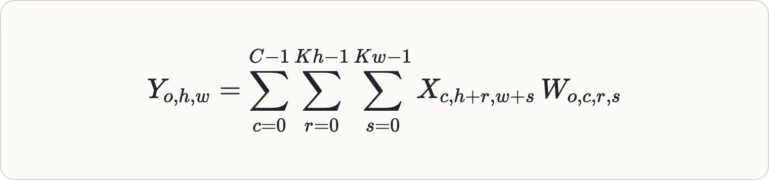
The running example is the 2D convolution a CNN computes, strictly a cross-correlation, written as a triple sum. Each output Y[o,h,w], for output channel o at row h and column w, adds up products over every input channel c and every kernel row r and column s: the input X at the window’s position times the weight W for that output channel. The typeset version on the left is how a paper prints it.

As a macro call it reads almost the same:

Y ← "Y[o,h,w] | O Ho Wo" ᵉe̲q< "sum c:=0..C - 1, sum r:=0..Kh - 1, sum s:=0..Kw - 1 | X[c,h+r,w+s] * W[o,c,r,s]"

The left string names the result, its free indices, and one extent for each, so the result has shape O Ho Wo; extents are written, never guessed. The right string is the sums, outermost first, each an operator word, an index and an inclusive range, then the summand after the bar. Inside the strings the notation is the paper’s: math precedence, brackets for indexing, and indices counted from 0 as the paper counts them.

Three macros parse the same text the same way:

Macro	Gives
ᵉe̲q<	the value, the array
ᵉt̲ex<	the LaTeX, a string
ᵉb̲oth<	both, as a pair

So the value and its typeset equation always describe the same thing. The library’s demo is one CNN layer, two 4 by 4 pictures through one 2 by 2 by 2 filter, with one call giving both:

"e:" u̲se< "Equations"
X ← 2 4 4 r̲eshape r̲ange 32
W ← 1 2 2 2 r̲eshape r̲ange 8
(C, Kh, Kw) ← (2, 2, 2)
(O, Ho, Wo) ← (1, 3, 3)
(Y, tex) ← "Y[o,h,w] | O Ho Wo" ᵉb̲oth< "sum c:=0..C - 1, sum r:=0..Kh - 1, sum s:=0..Kw - 1 | X[c,h+r,w+s] * W[o,c,r,s]"
"$$" c̲at tex c̲at "$$"
Y
Y m̲atch X ᵉc̲orrelate W

The demo as the library shows it: the program, and its output with the LaTeX line drawn as math. Click to enlarge.

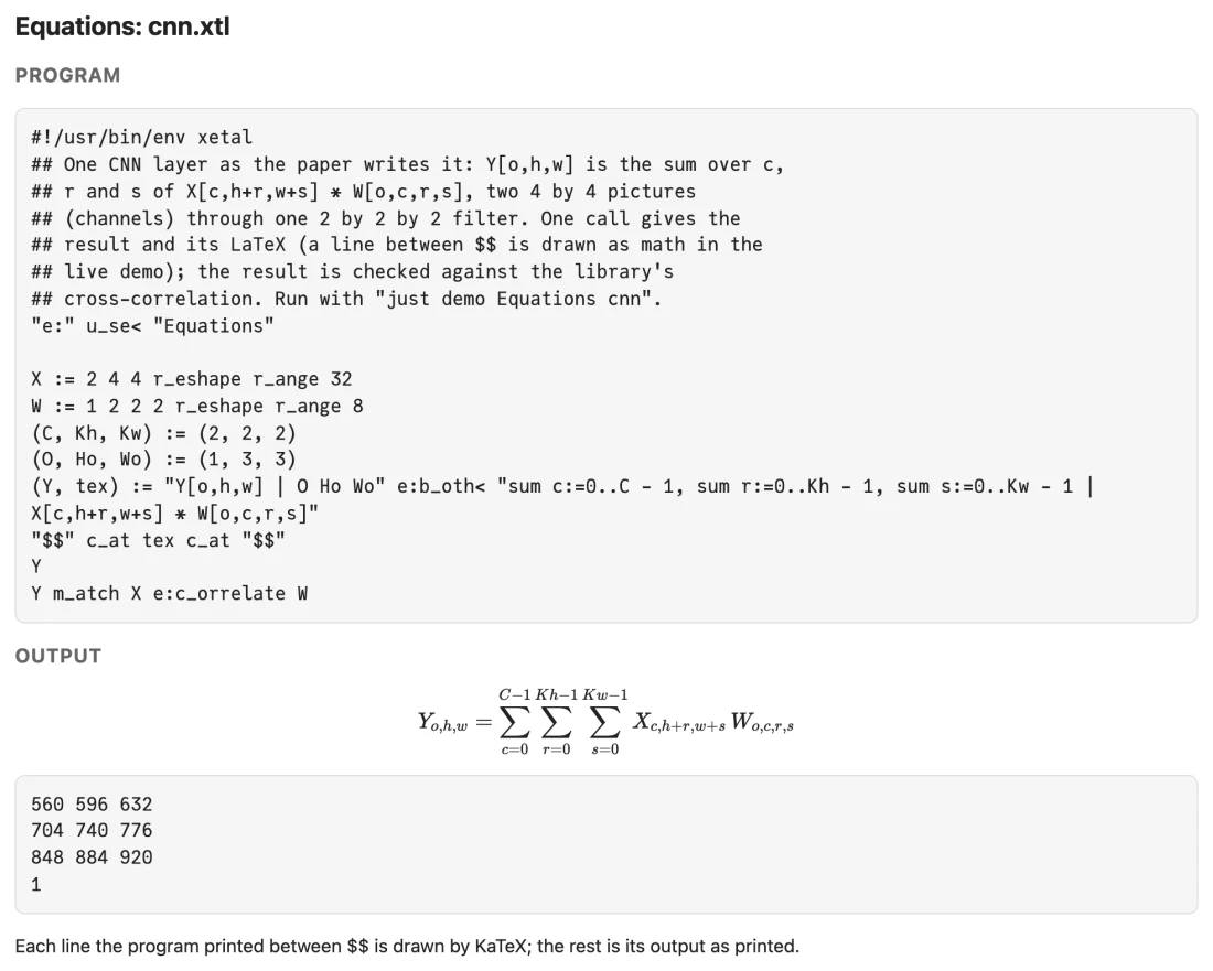
It prints the LaTeX between $$ markers, then the result, then a check:

$$Y_{o,h,w} = \sum_{c=0}^{C - 1} \sum_{r=0}^{Kh - 1} \sum_{s=0}^{Kw - 1} X_{c,h+r,w+s} \, W_{o,c,r,s}$$
560 596 632
704 740 776
848 884 920
1

The $$ line is for whatever shows the output. In the library’s live demo, and on the page just tex Equations cnn writes, shown here, that line is drawn as math by KaTeX; everywhere else it is plain text. The final 1 is the check: the result matches ᵉc̲orrelate, the library’s own cross-correlation, written a different way.

What it becomes

The macro writes ordinary X_eTaL, and xetal expand shows it. This is the demo’s call, expanded and rendered. The layout is the macro’s own: it writes its expansion as a program, one definition per line and each gather on its own line, so it can be read.

(Y, tex) ← ((({ @ →
  g3:a̲t ← { A i → (1 + i) s̲elect r̲avel A }
  g2:c̲heck ← { (A, name, k, from) e →
    n ← k s̲elect s̲hape A
    bad ← w̲here n̲ot r̲avel (0 ≤ e) ∧ e < n
    0 = t̲ally bad ? e
    "index" ⎕S̲IGNAL name c̲at " axis " c̲at (f̲ormat k) c̲at ": index " c̲at (f̲ormat (f̲irst bad) s̲elect r̲avel e) c̲at " is outside 0.." c̲at (f̲ormat n − 1) c̲at " (from " c̲at from c̲at ")"
  }
  g1:r̲ank ← { (A, name, q, ref) →
    (t̲ally s̲hape A) = q ? A
    "rank" ⎕S̲IGNAL ref c̲at " indexes " c̲at (f̲ormat q) c̲at " axes, but " c̲at name c̲at " has rank " c̲at f̲ormat t̲ally s̲hape A
  }
  g4:grid ← O c̲at Ho c̲at Wo
  g5:g̲rid ← { k → g4:grid r̲eshape (o̲ffsets k s̲elect g4:grid) 'l̲eft t̲able ('× r̲/ k d̲rop g4:grid) r̲eshape 0 }
  g4:grid r̲eshape (({ @ →
  g6:grid ← O c̲at Ho c̲at Wo c̲at (1 + (C − 1) − 0) c̲at (1 + (Kh − 1) − 0) c̲at (1 + (Kw − 1) − 0)
  g7:g̲rid ← { k → g6:grid r̲eshape (o̲ffsets k s̲elect g6:grid) 'l̲eft t̲able ('× r̲/ k d̲rop g6:grid) r̲eshape 0 }
  '+ r̲/₄ '+ r̲/₅ '+ r̲/₆ g6:grid r̲eshape ((
    ((g1:r̲ank (X, "X", 3, "X[c,h+r,w+s]")) g3:a̲t ((
      ((X, "X", 3, "w+s") g2:c̲heck ((0 + g7:g̲rid 3) + (0 + g7:g̲rid 6))) + (3 s̲elect s̲hape X) × (
      ((X, "X", 2, "h+r") g2:c̲heck ((0 + g7:g̲rid 2) + (0 + g7:g̲rid 5))) + (2 s̲elect s̲hape X) × 
      ((X, "X", 1, "c") g2:c̲heck (0 + g7:g̲rid 4)))))) × 
    ((g1:r̲ank (W, "W", 4, "W[o,c,r,s]")) g3:a̲t ((
      ((W, "W", 4, "s") g2:c̲heck (0 + g7:g̲rid 6)) + (4 s̲elect s̲hape W) × (
      ((W, "W", 3, "r") g2:c̲heck (0 + g7:g̲rid 5)) + (3 s̲elect s̲hape W) × (
      ((W, "W", 2, "c") g2:c̲heck (0 + g7:g̲rid 4)) + (2 s̲elect s̲hape W) × 
      ((W, "W", 1, "o") g2:c̲heck (0 + g7:g̲rid 1)))))))))
} @))
} @), "Y_{o,h,w} = \\sum_{c=0}^{C - 1} \\sum_{r=0}^{Kh - 1} \\sum_{s=0}^{Kw - 1} X_{c,h+r,w+s} \\, W_{o,c,r,s}"))

Each part maps back to the math:

• The outer block is the result’s own grid, O Ho Wo, one axis per free index, o, h and w.
• The inner block is the sum’s grid: the free indices again, then the summed ones, c, r and s, six axes in all. A sum is a term like any other, so it gets a block of its own, inside whatever it is part of.
• g̲rid k gives the value of the kth index at every point of a grid, so on the inner grid g̲rid 3 is w everywhere and g̲rid 6 is s.
• a̲t reads elements out of an array by flat position, a gather.
• The X term builds each flat position from the paper’s subscripts, w+s, h+r and c, combined by the array’s own dimensions, so X[c,h+r,w+s] becomes one gather over the whole grid. The W term does the same for W[o,c,r,s].
• c̲heck and r̲ank guard every gather: each subscript is checked against its axis, and each array against the number of subscripts written for it, with the text of the subscript kept for the message.
• '+ r̲/₄ '+ r̲/₅ '+ r̲/₆ are the three sums: reductions along the axes of c, r and s, leaving the O Ho Wo array that is Y.
• The g1: to g7: prefixes are fresh names the macro asks the language for, so nothing it defines can clash with a name in the program around it.
• The string at the end is the LaTeX, the second half of the pair that ᵉb̲oth< returns.

There are no loops in the result, just array operations, which is the same shape the GPU work in post #7 lowers to kernels.

Mistakes are caught where they can be. A malformed call is rejected when the macro expands, before the program runs; the library’s tests cover ten of them, among them a sum written c=0..C - 1 where c:=0..C - 1 is meant, a sum with no operator word, a missing summand, and an index bound twice:

"Y[o,h,w] | O Ho Wo" ᵉe̲q< "sum c:=0..C - 1, sum h:=0..1 | X[c,h,w]"
error[bad-equation]: an index is bound once: c, h, o, h, w

The rest is checked when the program runs, never left as a silent wrong read. Too few subscripts for an array:

error[rank]: X[c,h+r] indexes 2 axes, but X has rank 3

And an index outside its axis, here a sum that runs one past the two channels:

"Y[o,h,w] | O Ho Wo" ᵉe̲q< "sum c:=0..C | X[c,h,w]"
error[index]: X axis 1: index 2 is outside 0..1 (from c)

Beyond the CNN

Five more equations, typeset from the macro's own LaTeX, with what each computed. Click to enlarge.

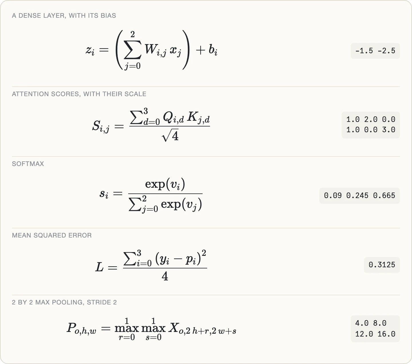
The convolution is the hardest case, three sums and arithmetic in the subscripts, but a sum is rarely the whole of an equation. A paper puts a bias after it, a scale or an average over it, and a function around its terms. So a sum in parentheses is a term like any other, max, min and prod join sum, and exp, log, sqrt, abs, max and min can be applied, spelled as a paper spells them. Five equations every model uses, each one call:

(z, tz) ← "z[i] | 2" ᵉb̲oth< "(sum j:=0..2 | W[i,j] * x[j]) + b[i]"
(S, tS) ← "S[i,j] | 2 3" ᵉb̲oth< "(sum d:=0..3 | Q[i,d] * K[j,d]) / sqrt(4)"
(s, ts) ← "s[i] | 3" ᵉb̲oth< "exp(v[i]) / (sum j:=0..2 | exp(v[j]))"
(L, tL) ← "L[] | " ᵉb̲oth< "(sum i:=0..3 | (y[i] - p[i])^2) / 4"
(P, tP) ← "P[o,h,w] | 1 2 2" ᵉb̲oth< "max r:=0..1, max s:=0..1 | X[o,2*h+r,2*w+s]"

• A dense layer, the weights W times the input x, then the bias b, added once, after the sum.
• Attention scores, each query in Q against each key in K, divided by the square root of the dimension, here 4.
• Softmax, each exponential over the sum of all of them.
• Mean squared error, the squared differences between targets y and predictions p, averaged. Its result names no index, L[], so it is a single number.
• Max pooling, the largest of each 2 by 2 window, stepping by 2: the stride is just arithmetic in the subscript.

The figure shows what each call returned, the LaTeX typeset and the value, and every value was checked by hand. The LaTeX follows the source: a quotient becomes a fraction, sqrt a radical, a parenthesized sum keeps its parentheses. Powers bind tightest, and a tower of powers is read from the top, as math reads it, so 2^3^2 is 512; the power comes before a minus sign, so -2^2 is −4. A name the grammar does not know, applied like a function, is refused rather than guessed at.

Checked against an oracle

The library was built test-first, against an oracle: ᵉc̲orrelate, the same cross-correlation written independently, with rotations, a transpose and one inner product. Three fixtures pin it. All ones gives 8 everywhere. X of 2 by 4 by 4 holding 0 to 31 and W of 1 by 2 by 2 by 2 holding 0 to 7 give the demo’s 1 by 3 by 3 result. And two output channels, three input channels and a 2 by 3 kernel on 5 by 6 pictures give a 2 by 4 by 4 result. The macro must match the oracle on all three, and it does.

The call’s form was not the first idea. The design compares seven ways of writing it, judged on whether a reader can see which bound goes with which index, whether different operators can mix, what a plausible slip does, how close it stays to the paper, and whether it works with no compiler change. The worst outcome is a slip that gives a silent wrong answer, and the chosen form, a binding per sum, was picked largely to rule those out.

What comes next

The library went from plan to finished in one evening, in five steps, each with its tests first: moving its copy of X_eTaL up to the current language, for fresh names and raw strings; the oracle; reading the call, with the rejections; the lowering, with the checks; and the LaTeX, with the demo and the documentation. Writing this post found a real bug, the worst kind: three summands that gave wrong answers with no error. (y[i] - p[i])^2 summed y - p, and y[i]2 and y[i] % 2 summed y, while the LaTeX printed what was written. The reader had used part of its text and dropped the rest. It was fixed the same morning: every rule of the grammar now uses all of its text or refuses the call, only the grammar’s own characters may appear, and ^ joined the grammar. Each of the three is now a test. And as a guard for the whole class, every call is now read three ways from one grammar, as the value, as the LaTeX and as a plain reprint, and the reprint is compared with the text as written: a rule that dropped a character would make them differ, and the call is refused.

Then I asked for readable expansions: the macro now lays its expansion out as a program, as shown above, and xetal expand now does the same for every macro. And one name changed before this post: the value macro was q_<, which read as “eq” only beside the alias e:. Since the alias is the caller’s choice, it is now e_q<, which reads as “eq” under any alias, like its siblings t_ex< and b_oth<. Macros also had a bug, which I hit in X_eTaL’s live demo: with its Boxed display on, every macro call in every program failed, because a macro’s expansion went through the same printer as the program’s output and came back drawn as a box instead of as source. That is fixed, with tests that were red before the fix.

Still ahead for equations: the parts deliberately left out, padding and dilation for convolutions, and a shape check, planned in X_eTaL, that catches a wrong shape before a program runs rather than after. And because every macro that reads a notation is a parser, the readers’ rule, use all of the text or refuse it, is becoming a parsing library of its own for macro writers, the subject of a planned post. Anything a macro cannot cover is reviewed and decided, never assumed.

Sums are not the only operator an equation needs. A continuous convolution is an integral, and integrals are planned as well, with the numerical method stated in the program rather than assumed; they too are the subject of a planned post.

Equations are one half of the notation ML needs. The other is the data flow a model runs, layer after layer, which reads left to right where X_eTaL reads right to left; a pipeline macro for it is the subject of a planned post. Both lower to ordinary X_eTaL, so what they produce can run on the GPUs of post #7, through OpenCL or, as of post #10, Mojo, and be drawn step by step in Blender, as the softmax and matrix-product videos in post #9 already are.

---

[Ed. 2026/10/17: the table of the three macros now shows them rendered, ᵉe̲q<, ᵉt̲ex< and ᵉb̲oth<, as the rest of the post does, rather than as typed (e:e_q<, ...). This post's history.]